Subtyping patients based on cortical atrophy patterns through the Louvain method
(2015-2017: Last Update: March 10, 2017)
(2015-2017: Last Update: March 10, 2017)
Description
This is a MatLab library for clustering patients with similar cortical atrophy pattern using the Louvain method for modular organization extraction.
We used its implementation in the Brain Connectivity Toolbox. Thus, to run our codes, please download it here.
Here, we briefly describe the method and how to install and use with a simple example.
For the thorough description, please refer the paper below.
(related paper: Robust Identification of Alzheimer’ Disease subtypes based on cortical atrophy patterns, JY Park, HK Na, SS Kim, HW Kim, HJ Kim, SW Seo, DL Na, CE Han, JK Seong, Scientific Reports 2017)
If you find any error or have any suggestion, please contact us. (Jong-Yun Park or Cheol E. Han).

Our analysis consists of three steps: estimating cortical atrophy pattern, computing a similarity matrix between subjects, and clustering with the Louvain method.
Estimating cortial atrophy map
To estimate the cortial atrophy, we use z-scores of cortical thickness normalized by the distribution of cortical thickness in the CN group, instead of using raw cortical thickness. The raw cortical thickness is a snapshot of the current remnants; however, for the cluster analysis of the cortical thinning pattern, it is better to measure the extent of cortical atrophy in each patient instead. Generally, it is not possible to observe the extent of cortical thinning within a single MR image, as we cannot determine the cortical thickness of the brain before AD diagnosis. In this study, we estimated the level of cortical atrophy by normalizing the remnant cortical thickness with the distribution of cortical thickness in the CN group. The standard deviation for each brain region may account for inter-subject variability; in cases where large inter-subject variability resides, even when the remnant is small, it would not be considered as severe cortical atrophy (Figure 1). Since this procedure considers the inter-subject variability, where the large inter-subject variability lies, the resultant z-score is not low even when the subject\u2019s cortical thickness is thinner than the mean of the CN subjects. Thus, in the resultant cortical atrophy patterns, the deep or shallow atrophy is determined not only by the cortical thinning of the patient, but also by the inter-subject variability in the CN group. We believe that the use of this z-score improves subtyping performance.
Computing a similarity matrix between subjects
Our subtyping strategy utilizes correlation coefficients which tends to cluster AD patients into distictive subtypes in which patients share similar cortical atrophy pattern regardless the overall depth of cortical atrophy and thus may perform better than approaches based on Euclidean distance. This superiority arises from the nature of the correlation coefficient itself in that the absolute values of cortical thickness can be automatically controlled in the operation process and thus using correlation coefficients is useful to capture similarities in cortical thinning patterns between the two subjects, rather than the differences in thickness, and is therefore more sensitive in distinguishing the pattern difference.
Clustering with Louvain method
Finally, we employed the Louvain method which was developed for modular organization extraction in network science. The modular organization in a large network can be found by maximizing a value of modularity which is high when the intra-modular connections are dense while the inter-modular connections are sparse. The Louvian method is the current state-of-the-art method for modular organization extraction. In our problem setting, dense inter-modular connections imply high similarity of the cortical atrophy pattern between subjects in a module. The Louvain method is not only efficient for larger networks, but also very accurate; for a few large networks, its value of modularity was the highest among the current common modular organization extraction methods.
Install Brain Connectivity Toolbox for MatLab.
Download our subtyping package.
Unpack anywhere you prefer.
Launch matlab.
Add the paths where you unpack the library by typing the following in the matlab commandline.
Or you may use the menu of the MatLab GUI.
addpath /home/user/matlab/BCT/
addpath /home/user/matlab/subtyping_louvain/
Download our example data [1] [2].
(OPTIONAL) Install SurfStats Toolbox for MatLab.
(related paper: Robust Identification of Alzheimer’ Disease subtypes based on cortical atrophy patterns, JY Park, HK Na, SS Kim, HW Kim, HJ Kim, SW Seo, DL Na, CE Han, JK Seong, Scientific Reports 2017)
If you find any error or have any suggestion, please contact us. (Jong-Yun Park or Cheol E. Han).
Our analysis consists of three steps: estimating cortical atrophy pattern, computing a similarity matrix between subjects, and clustering with the Louvain method.
Estimating cortial atrophy map
To estimate the cortial atrophy, we use z-scores of cortical thickness normalized by the distribution of cortical thickness in the CN group, instead of using raw cortical thickness. The raw cortical thickness is a snapshot of the current remnants; however, for the cluster analysis of the cortical thinning pattern, it is better to measure the extent of cortical atrophy in each patient instead. Generally, it is not possible to observe the extent of cortical thinning within a single MR image, as we cannot determine the cortical thickness of the brain before AD diagnosis. In this study, we estimated the level of cortical atrophy by normalizing the remnant cortical thickness with the distribution of cortical thickness in the CN group. The standard deviation for each brain region may account for inter-subject variability; in cases where large inter-subject variability resides, even when the remnant is small, it would not be considered as severe cortical atrophy (Figure 1). Since this procedure considers the inter-subject variability, where the large inter-subject variability lies, the resultant z-score is not low even when the subject\u2019s cortical thickness is thinner than the mean of the CN subjects. Thus, in the resultant cortical atrophy patterns, the deep or shallow atrophy is determined not only by the cortical thinning of the patient, but also by the inter-subject variability in the CN group. We believe that the use of this z-score improves subtyping performance.
Computing a similarity matrix between subjects
Our subtyping strategy utilizes correlation coefficients which tends to cluster AD patients into distictive subtypes in which patients share similar cortical atrophy pattern regardless the overall depth of cortical atrophy and thus may perform better than approaches based on Euclidean distance. This superiority arises from the nature of the correlation coefficient itself in that the absolute values of cortical thickness can be automatically controlled in the operation process and thus using correlation coefficients is useful to capture similarities in cortical thinning patterns between the two subjects, rather than the differences in thickness, and is therefore more sensitive in distinguishing the pattern difference.
Clustering with Louvain method
Finally, we employed the Louvain method which was developed for modular organization extraction in network science. The modular organization in a large network can be found by maximizing a value of modularity which is high when the intra-modular connections are dense while the inter-modular connections are sparse. The Louvian method is the current state-of-the-art method for modular organization extraction. In our problem setting, dense inter-modular connections imply high similarity of the cortical atrophy pattern between subjects in a module. The Louvain method is not only efficient for larger networks, but also very accurate; for a few large networks, its value of modularity was the highest among the current common modular organization extraction methods.
important note
Since the Louvain method is based on a greedy optimization method, the clustering results can vary slightly. To resolve this issue, we employed a ‘major voting’ scheme, in which we extracted modular organization N times, and labeled a subject with the most frequently assigned cluster. The Louvain method has a resolution parameter, γ (gamma), which controls the number of clusters.
Since the Louvain method is based on a greedy optimization method, the clustering results can vary slightly. To resolve this issue, we employed a ‘major voting’ scheme, in which we extracted modular organization N times, and labeled a subject with the most frequently assigned cluster. The Louvain method has a resolution parameter, γ (gamma), which controls the number of clusters.
(OPTIONAL) Visualization of cortical atrophy
We compared the cortical thickness data of subtype group with that of CN using a 2-sample t-test with random field theory using SurfStat (http://www.math.mcgill.ca/keith/surfstat). We also visualized the cortical atrophy pattern using SurfStat. Since our subtyping methods clustered subjects based on the cortical atrophy pattern not the level of overall cortical thinning, the distribution of cortical atrophy of each vertices did not follow the normal distribution. Thus we visualized the median of cortical atrophy as a cortical atrophy map.
We compared the cortical thickness data of subtype group with that of CN using a 2-sample t-test with random field theory using SurfStat (http://www.math.mcgill.ca/keith/surfstat). We also visualized the cortical atrophy pattern using SurfStat. Since our subtyping methods clustered subjects based on the cortical atrophy pattern not the level of overall cortical thinning, the distribution of cortical atrophy of each vertices did not follow the normal distribution. Thus we visualized the median of cortical atrophy as a cortical atrophy map.
How to install
Or you may use the menu of the MatLab GUI.
addpath /home/user/matlab/subtyping_louvain/
How to use
This package has two functions. estimate_cortical_atrophy and community_louvain_major_vote. See below for the example.
estimate_cortical_atrophy
AD_thickness, CN_thickness |
thickenss matrix which size is m x n (m: number of subjects, n: vertex of thickness)Their column sizes which mean vertex of thickness should be identical. | |
Z score |
Z score matrix of thickness to be normalized (m x n matrix; m: number of subjects, n: vertex of thickness) |
community_louvain_major_vote
=community_louvain_major_vote(similarity matrix, [gamma, repetition]);
similarity matrix |
similarity matrix between nodes (subjects) (a m-by-m matrix where m is the number of subjects.)γ (gamma) | |
γ (gamma) |
a resolution parameter. The value lower than one will make the lesser number of clusters which means larger sized clusters (Default: 1). | |
repetition |
the nubmer of repetition time (Default: 1000). | |
cluster_index |
The primary output of the function. subtype labels for each node (each subject) (a m-lengthed vector). | |
confidence |
The value which shows how consistently each node (each subject) belongs to clustered subtype in major voting. (a m-by-repetition matrix). | |
Q |
modularity value whose maximum value is 1. | |
cluster_all |
esults of all repeated cluster estimations. This code is a rough implementation. It only works when the modular organization is not quite varying. VISUAL CHECK OF MAJOR VOTING RESULTS IS RECOMMENDED using the following command. |
cluster_mapping
idx1, idx2 |
cell-type variables which contains subjects of each modular organization. For example, idx1={[1,2],[3,4]} means two modules with two subjects each. | |
score |
accuracy score which represent how well two modular organization are matched. | |
omap |
overlapping map. m-by-n intersect matrix where m is number of modules in idx1 and n is number of modules in idx2. Each element of (i,j) contains the number of overlapped subjects between the ith module of idx1 and jth module of idx2. | |
m_idx |
matching table from idx1 to idx2 |
draw_reordered_similarity_matrix
similarity_matrix |
a m-by-m matrix where m is number of subjects | |
Ci |
cluster index (a m lengthed vector). | |
similarity_reordered |
m-by-m matrix of reordered similarity_matrix |
Example
We first estimated cortical thickness of Alzheimer's Disease and normal control (CN) using FreeSurfer.
We resampled and filtered the cortical thickness with the Laplace-Beltrami operators following
our previous paper. Computing the cortical thickness, resampling and filtering with the Laplace-Beltrami operator is beyond the scope of this example. Instead, we prepared the resampled and filtered cortical thickenss in the example data.
1. Load the prepared dataset (type the following lines in matlab commadline)
load (dataset_name).mat
AD_thk=[Subtype_AD.lb_lh, Subtype_AD.lb_rh];
AD_thk=AD_thk.*repmat(cortex_mask,[size(AD_thk,1),1]);
NC_thk=[Subtype_NC.lb_lh, Subtype_NC.lb_rh] ;
NC_thk=NC_thk.*repmat(cortex_mask,[size(NC_thk,1),1]);
load (dataset_name).mat
AD_thk=AD_thk.*repmat(cortex_mask,[size(AD_thk,1),1]);
NC_thk=[Subtype_NC.lb_lh, Subtype_NC.lb_rh] ;
NC_thk=NC_thk.*repmat(cortex_mask,[size(NC_thk,1),1]);
2. Estimate the cortical atrophy by computing Z-score of cortical thickness normalized by the distribution of cortical thickness in the CN group using the following command.
[AD_mwr]=estimate_cortical_atrophy(AD_thk, NC_thk]);
[AD_mwr]=estimate_cortical_atrophy(AD_thk, NC_thk]);
3. Compute Similarity matirx by Pearson correlation coefficients between atrophy patterns of any two subjects.
similarity_matrix=corr(AD_mwr');
similarity_matrix=corr(AD_mwr');
4. Subtyping using the computed similarity matrix and the Louvain method.
In this example, as we did in the paper, we set gamma value 0.9 and repetetion of major voting as 1000.
[Ci, confidence, meanQ]=community_louvain_major_vote(similarity_matrix, 0.9, 1000);
In this example, as we did in the paper, we set gamma value 0.9 and repetetion of major voting as 1000.
[Ci, confidence, meanQ]=community_louvain_major_vote(similarity_matrix, 0.9, 1000);
5. Draw the reordered simialarity matrix to confirm the clustering results.
draw_reordered_similarity_matrix(similarity_matrix, Ci)

draw_reordered_similarity_matrix(similarity_matrix, Ci)
6. (OPTIONAL) Visualize the cortical atrophy map using the following commands.

a) Load the prepared dataset and perform smoothing over each hemisphere surfaces.
[coord1,tri1]=load_surf_obj('lh.pial.mean.obj');
[coord2,tri2]=load_surf_obj('rh.pial.mean.obj');
tri2=tri2+40962;
surf.tri=[tri1;tri2];
surf.coord=[coord1;coord2]';
Y = SurfStatSmooth( surf.coord, surf, 20 );
s100smooth.coord = Y( :, :, 1 );
s100smooth.tri = surf.tri;
mask=logical(cortex_mask);
b) Compute statistical difference between CN and AD in cortical thickness.
SurfStatLinMod find linear model, at this case two linear models each represent CN and AD, and SurfStatT gives T statistic for CN-AD cortical thickness
thick_NC=NC_thk;
thick=[AD_thk(g_idx{j},:)];
Grp=cellstr([repmat('NC',[size(thick_NC,1),1]);repmat('AD',[size(thick,1),1])]);
glb_grp=term(Grp);
glb_thk=[thick_NC;thick];
contrast=glb_grp.NC-glb_grp.AD;
slm = SurfStatLinMod( glb_thk,(glb_grp) , surf);
slm = SurfStatT(slm,contrast);
Y = SurfStatSmooth( [mean(thick);slm.t], surf, 10 );
slm2=slm;
slm2.t=Y(2,:);
[coord2,tri2]=load_surf_obj('rh.pial.mean.obj');
tri2=tri2+40962;
surf.tri=[tri1;tri2];
surf.coord=[coord1;coord2]';
Y = SurfStatSmooth( surf.coord, surf, 20 );
s100smooth.coord = Y( :, :, 1 );
s100smooth.tri = surf.tri;
mask=logical(cortex_mask);
SurfStatLinMod find linear model, at this case two linear models each represent CN and AD, and SurfStatT gives T statistic for CN-AD cortical thickness
thick_NC=NC_thk;
thick=[AD_thk(g_idx{j},:)];
Grp=cellstr([repmat('NC',[size(thick_NC,1),1]);repmat('AD',[size(thick,1),1])]);
glb_grp=term(Grp);
glb_thk=[thick_NC;thick];
contrast=glb_grp.NC-glb_grp.AD;
slm = SurfStatLinMod( glb_thk,(glb_grp) , surf);
slm = SurfStatT(slm,contrast);
Y = SurfStatSmooth( [mean(thick);slm.t], surf, 10 );
slm2=slm;
slm2.t=Y(2,:);
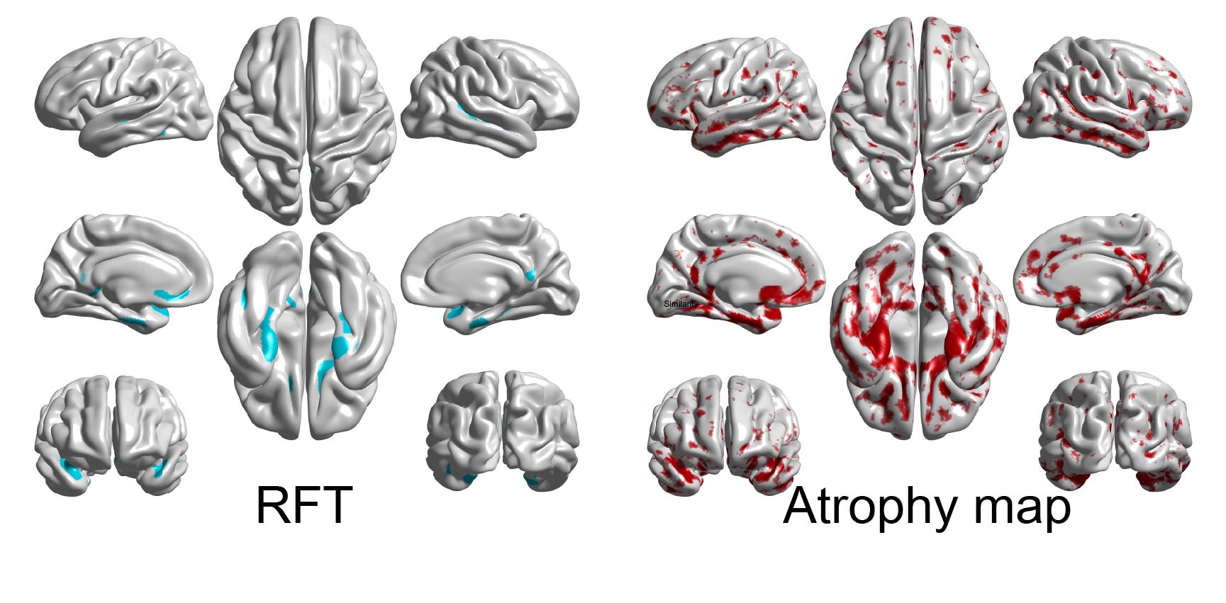
c) Estimate corrected p-values for each cluster using the random field theory (RFT) with SurfStatP. Cyan shows clusters whose corrected p-values is under 0.05, and yellow-red represents p-values of peaks for the clusters
[Pval,peak,clus]=SurfStatP( slm2 ,mask, 0.001);
[~,cb]=SurfStatView( Pval.C, s100smooth, 'corrected P' );
[Pval,peak,clus]=SurfStatP( slm2 ,mask, 0.001);
[~,cb]=SurfStatView( Pval.C, s100smooth, 'corrected P' );
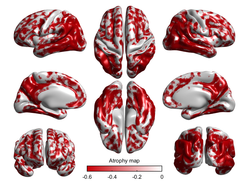
d) Draw an atrophy map which shows medians of the cortical atrophy (z-scores) in each subtype using the following commands (-0.6<=z<=-0.3)
temp_thk=median(AD_mwr(g_idx{j},:));
temp_thka=temp_thk;
temp_thka(temp_thk>-.3)=0;
temp_thka(temp_thk<-.6)=-.6;
[~,cb]= SurfStatView( temp_thka, s100smooth,'Atrophy map' );
temp_thk=median(AD_mwr(g_idx{j},:));
temp_thka=temp_thk;
temp_thka(temp_thk>-.3)=0;
temp_thka(temp_thk<-.6)=-.6;
[~,cb]= SurfStatView( temp_thka, s100smooth,'Atrophy map' );
SCBIA Lab. Korea University. Republic of Korea.